src: AGUvideos
Friday, December 14, 2012
Friday, December 7, 2012
4179 Toutatis Close Approach to Earth
The Near Earth Asteroid 4179 Toutatis will make a close approach to the Earth on Dec 12, 2012 at 6:40 am (UT) according to an ephemeris generated by JPL's HORIZONS website. A summary of the data in the ephemeris is given in the following table.

I loaded the orbital elements for Sep. 30, 2012 into Distant Suns and got the position indicated by the small white + for the time of close approach. The red marker shows the HORIZONS coordinates from the table above. The orbit may have been perturbed by the asteroid's proximity to the Earth. The perihelion longitude is ϖ=Ω+ω where Ω is the angle of the Ascending Node or the angular distance along the equator from the Vernal Equinox to the point where the orbit crosses the equator and ω is the argument of perihelion which is the angle from the equitorial plane to the asteroid's perihelion in the plane of its orbit. The asteroid's path is roughly parallel to the Ecliptic (the diagonal line through Pisces) but shows maximum deviation from it at the time of close approach. The apparent magnitude at close approach is given as 10.86 which means that one will need a telescope to see it.

Thursday, December 6, 2012
AGU 2012 - DEEPSEA CHALLENGE (Cameron)
James Cameron spoke at AGU 2012 about his dives in the Deepsea Challenger in which he made a descent to a depth of nearly 36,000 ft. The videos shown in the talk were copyrighted and so part of the presentation was blocked. Here are some links to help fill in the gaps: steel sphere syntactic foam pelagic sea cucumber (holothurian)
src: AGUvideos
AGU 2012 - Watson Presentation
The AGU 2012 Frontiers of Geophysics Lecture by Sir Robert Watson focused on gobal warming. He said that we will probably not make the 2°C goal for global warming but that a 5°C world would be more likely. Other conclusions were that reducing green house gases was a management issue. The world price for rice in a warmer world would increase due to reduced productivity and greater demand. We would have to depend more on renewable energy but that would not be enough and so we might have to rely more on nuclear energy but the damage to the Japanese reactor as a result of the tsunami would hinder progress in that direction. The current growth in CO2 emissions is primarily due to China's contribution while emissions in the US and Europe have been relatively constant but he also noted that the US has the highest contribution per person.
Wednesday, December 5, 2012
New Multi-Year Mars Program
NASA is proposing a new rover similar to Curiosity to be sent to Mars in 2020. Plans include a camera with a telescopic lens [which might be used to do a little astronomy]. NASA administrator John Grunsfeld talked the new multi-year Mars program about the future of Mars exploration at yesterday's AGU 2012 conference.
src: nasajpl2
Monday, December 3, 2012
MSL Dec 3 Press Conference at AGU 2012
src: nasajpl
Today's MSL Press Conference was held at a new venue, the AGU 2012 Fall Conference in San Francisco. It was a recap of Curiosity's progress on Mars to date and revealed a little more about recent SAM, Sample Analysis at Mars, results. Curiosity will stay in the Glenelg area for about another month and then she will start heading towards Mt Sharp and get started on the main science mission. One task remaining in her engineering checkout is the drill test which will be done a new location, Yellow Knife Bay. The major SAM result is the high ratio of deuterium to hydrogen, D/H, found in the evolved gases from the fifth Rocknest scoop and some simple chlorinated methane molecules. A high D/H ratio can be attributed to a loss of hydrogen in the Martian atmosphere over time either into space or through some surface process. The main gases detected by the SAM instrument are H20, CO2, O2 and SO2.
Supplemental (Dec 5): related press release with the AGU 2012 MSL press conference images.
Wednesday, November 28, 2012
Amateur Astronomy on Mars?
The country is currently facing automatic budget cuts in January known as sequestration if Congress doesn't come up with some stopgap measures. This means that public support for the Mars programs will be cut proportionally. This will not decrease the functionality of the Mars rovers but their controllers might feel the pinch. One possiblity that NASA might consider is more private support and some "amateur work."
As an example Curiosity might try some amateur astronomy with the M-100 Mastcam. It has a focal length of 100mm with an f/10 lens and can capture 1600x1200 6.8°x5.1° images. So, time permitting, it might be possible for Curiosity to observe the location of the Martian rotational pole. In Curiosity's case it would probably have to be the South Celestial Pole. A complicating factor is that Curiosity is in a depression about 5° S of the equator so the pole would be very close to the horizon in a dusty environment. But the visible star trails that result from the rotational motion of Mars might still be useful in determing the location of the South pole even if it is not clearly visible. The S pole is diagonally opposite the N pole so it is at RA 9h10m44s, Decl -52°53'11.4" and there are some bright stars nearby in the constellation Vela that could be used to triangulate the pole's position. In the image below one can see the marked position of the S pole and the surrounding stars of Vela.

Monday, November 26, 2012
North Celestial Pole 03b
I again used the rotation center formula to calculate the pixel position of the center of rotation in the image using the pairs of points within 1000 pixels of the approximate center. The root mear square error for the pair distances from the center was 1.59 pixels. The RA and Decl are known for α UMi and λ UMi and they can be used to obtain a scale factor which can be used to convert pixel separations to angular distances.

Letting e be a unit vector representing the position of a star and using the formula equating the dot product of two positions to the cosine of the angle between them we get two conditions for direction of the pole. Each condition specifies a circle on the celestial sphere with the known angular distance of the pole from the star. We can represent the circle about λ UMi by an equation for a circle on the sphere.

The second condition tells us that the position of the pole is a zero of a nonlinear equation which can be plotted to estimate the angles for the zeros.

Substituting the equation for the circle from the first condition into the second condition we get a simple equation which is linear in terms of the sine and cosine of an angle that can be solved for an expression for the sine of the unknown angle.

Plugging the constants into the expression gives the sine of the angle, the angle and the direction of the pole in Cartesian coordinates.

We can now calculate the Right Ascension and Declination of the computed pole in the J2000 coordinate system.

Twelve years have elapsed since the year 2000 and we can expect some movement of the pole due to precession and nutation. The observed pole is about 9 arc minutes from the J2000 pole. The expected error in the observed pole is about 14 arc seconds.
North Celestial Pole 3a


I zoomed in on the pole a little more Saturday evening and was able to see more of the fainter stars near the pole. The bright star at the top of the image is Polaris, α UMi, and the brighter star towards the bottom center is λ UMi. If you look slightly above and to the left of Polaris you will see a small star and a much smaller companion which is an optical binary. Some of the stars just visible are approximately 9th magnitude.
The second image is a merger of 6 images taken approximately 8 minutes apart. With greater magnification one has to be more careful about camera motion. If you look carefully at the rotational track you will see that one of the stars is out of alignment. It was not used to determine the center of rotation which is marked with a +.
These images are approaching the limit of what one can do with a digital camera with 26X optical zoom. Magnification reduces the speed of the lens so longer exposure times or a larger aperature is needed. One could probably improve on the position of the pole by using zooming in more with a good telescope.
Friday, November 23, 2012
Distant Suns Star Chart

The above image is approximately the same field of view in Distant Suns as the images taken on Wed evening. The white lines mark the angles of Right Ascention corresponding to 0h at the top and 6h, 12h and 18h going clockwise. Part of the handle of the Little Dipper is also marked. The closest star on the handle is δ UMi (mag. 4.35)and the one just visible at the edge of the image is ε UMi. (mag. 4.21). All the stars visible in this star chart are greater than magnitude 7. To give a sense of scale ε UMi is about 8° from the pole.
Thursday, November 22, 2012
North Celestial Pole 2

On Wednesday evening I captured several images of the North Celestial Pole like the one above. Each image was 4288 x 3216 and the exposure was 16 seconds with an F-Stop of 4.5. Six of the images taken about 8 minutes apart were merged and the ends of the arcs were used to calculate the pole using the formula for the rotational center. My results agreed fairly well with the J2000 position. The humidity was about 75% and there was some sky glow present. The brightest star near the center is Polaris.

Supplemental (Nov 22): I've replaced the original merged image which used the sum of the pixel values of the image points with one that uses the greater of the two pixel values. There's a little more background noise but the pixel values are more representative of the observations. The images posted are one sixth the size of the originals. MS Paint was used to get the pixel coordinates for the data. The "+" marks the computed pole position.
Friday, November 16, 2012
Locating the North Celestial Pole

The formula used to find the center of a circle can be used for other applications as well. The formula computes a position that will minimize the difference between pairs of points. The radial distance from the center does not have to be the same for each pair. This will enable us to calculate the position of the North Celestial Pole on an image using the endpoints of a streak formed by the motion of a star. The calculation of the center of rotation is shown below.

Thursday, November 15, 2012
Checking Event Times With Mars24
One can view the position of Mars for a specific date and time on the Mars24 plots by using the Settings tool found in the Window drop down menu. The orbit and analemma plots for perihelion are shown below. Ls in the analemma plot appears to be the Sun's RA given in degrees of longitude and is used in place of a date.


Supplemental (Nov 19): The Mars24 technical notes state that Ls is the areocentric longitude of the Sun measured from the Martian equinox. This is probably the relative longitude along the celestial great circle of the Martian ecliptic due to the Sun's motion in its "areocentric orbit." Ls is also used in connection with the ephemeris time (ET).
Nov 15th MSL Teleconference
src: nasajpl
Today's telecon dealt primarily with Curiosity's local environmental conditions such as dust devils, pressure fluctuations and radiation levels. The pressure fluctuations not only exhibit daily changes but also changes over a longer timeframe. Mars is currently moving closer to the Sun and will reach perhelion on Jan. 23, 2013*. The radiation on Mars is more easily affected by its environment in space since it has lost its magnetic field and has a relatively thin atmosphere as compared with Earth conditions. The radiation levels fluctuate during the day and are greatest when the atmospheric pressure is lowest. The local winds also fluctuate throughout the day and move up slope on Mt Sharp and Gale Crater's rim during the day and down slope at night. Curiosity is near the center of these two flows and is in the region where winds flow around Mt Sharp. related press release telecon images Timekeeping on Mars Mars24 Sunclock
*Supplemental (Nov 15): MICA's perihelion is 2013 Jan 24 08:56 UT
MSL on NOVA
Watch Ultimate Mars Challenge on PBS. See more from NOVA.
Some background on the development of the Mars Science Laboratory rover Curiosity was shown on the PBS program NOVA Wednesday evening.
Monday, November 12, 2012
Total Solar Eclipse

There will be a total solar eclipse on Tues. Nov 13, 2012. Unfortunately the only major landmass for which totality will be visible will be the northernmost part of Australia. The eclipse will start at 19:38 UT and end at 0:46 UT. see details
Tuesday, November 6, 2012
Estimated Circle Center & Radial Residuals
I may have violated my position on avoiding misnomers in the last blog. The residuals there would more correctly called radial pair differences. With an estimated center for the circle one can compute a mean radius for the initial points and a better set of radial residuals as well as their rms error. The expected error in the mean radius would be εrms/√5=0.173. Half the radial errors would have a magnitude less than 0.512 pixels as might be expected when working with integers.

Friday, November 2, 2012
More on the Least Squares Estimate of a Circle's Center
The formula for the least squares estimate for the center of a circle that was used in a recent blog uses the difference in the square of the distance from the center for pairs of points as the difference whose square is to be optimized. One can study how the formula works for different sets of pairs of points. A path can be drawn between the original five points that will link all the 10 pairs of points in a sequence. The first two pair of points with the largest separation gives the center of the circumscribed circle through the set of three points. The same is true for the three pair pairs of points for the triangle with the largest sides. As one adds more pairs of points the estimated center is less dependent on the individual points used and tends to converge but there is some residual difference between the distance of a point from the center for the pairs. Squares of the distance of a point from the center were used to compute the differences to avoid the use of square roots in deriving the formula. The method is similar to using hyperbolic navigation to determine one's position.


Supplemental (Nov 2): I got residuals that differed in the third decimal place from the radial residuals for the 10 pair of points above using a method for determining position based on differences in signal arrival times. The data points for the circle were treated as signal sources whose positions were known and the differences in arrival times were set to zero. The estimated position of the center also differed in the third decimal place.
Nov 2nd MSL Telecon: Negative Result for Methane on Mars
src: nasajpl
Today's MSL teleconference focused on the SAM suite of instruments used to study the composition of gases in the Martian atmosphere and the presence of volatile compounds from the surface. The Tunable Laser Spectrometer is can measure the isotopic composition of the carbon compounds in the atmosphere. The relative abundance of the isotopes present can give information on the escape of gases from the Martian atmosphere over time. Heavier isotopes are less likely to escape which results in a higher abundance. The instument was not able to detect the presence of methane in the atmosphere. The conclusion is that if there is any methane present the sinks on the surface dominate over the sources. telecon images related press release
Thursday, November 1, 2012
MSL's 1st X-ray Diffraction Pattern (1D)
I tried to convert MSL's first 2D diffraction pattern to a 1D pattern. The first problem is to find the center of the pattern of rings. This was done by doing a least squares fit for five pixel points on one of the rings. The calculation goes as follows.

One can check the fit by plotting a circle on the 2D diffraction pattern.

A 1D diffraction pattern was obtained by measuring the distances of the image pixels from the center of the rings and summing the gray scale image values for the radii in one pixel intervals and then dividing by the number of pixels in each interval to get average values.

The peaks in the 1D plot can be compared with powder diffraction databases to determine the minerals present. For more information on XRD and CheMin see the MSL Science Corner and David Blake's Historical Perspective.
Tuesday, October 30, 2012
Oct 30th MSL Teleconference
src: nasajpl
At Tuesday's teleconference the MSL project scientists discussed the results of the first xray diffraction measurements made on another body of the solar system. Using xray diffraction equipment that had been reduced from the size of a refrigerator on Earth to that of a shoe box for the mission they were able to capture the diffraction pattern of finely divided particles to determine the minerals present. The minerals were basaltic and similar to feldspar, pyroxene and olivine. The particles are believed to be a mixture of blown in dust and local particles along with volcanic glasses and their weathered products. telecon images and related press release
Sunday, October 28, 2012
Earthquake Convictions in Italy 2
The plots in the last blog may not be admissible as evidence against the individuals charged with wrong doing since they assume facts not in evidence at the time the statements were made, specifically, the existence and time of the M6.3 earthquake. Here is a new set of plots using averaging intervals of 1/3 of the anomalistic month of 27.55 days. They start at the beginning of 2002 and the time scale is in Julian years of 365.25 days.


There doesn't appear to be much to indicate that a major earthquake is imminent. There is a decrease in the frequency of earthquakes in an interval of time and some low level earthquakes are missing. The pattern of the total energy of the earthquakes in an interval for several years before the earthquake doesn't appear to change much. The nonuniformity could be interpreted as statistical fluctuations as might be the increase in the average energy with fewer earthquakes per interval. With lower numbers one can expect greater fluctuations in the average. What may be abnormal is the low level of earthquake activity immediately prior to the time of the major earthquake which I have referred to elsewhere as a "lull." Another oddity is the disappearance of low level earthquakes which might indicate that the faults have locked up some. It's still difficult to point to anything that says there will be a major earthquake soon.
Supplemental (Oct 28): One should probably ask if the absence of earthquakes below M2.5 from mid 2004 onward was due to a change in earthquake activity or a change in monitoring them. Would a global network charged with monitoring earthquakes worldwide reduce the sensitivity of a seismograph when there are a large number of local earthquakes or would they reduce the number reported to the system? The explanation might be relevant to the case.
Saturday, October 27, 2012
Earthquake Convictions in Italy
Six scientists and a former government official were found guilty in an Italian regional court on October 22 for making "inaccurate, incomplete and contradictory" statements prior the the magnitude 6.3 earthquake in Aquila on April 6, 2009. I downloaded the data for the earthquakes with magnitudes greater than 2.0 from the beginning of 2002 to just prior to the M6.3 earthquake and within 1 degree in latitude and longitude of l'Aquila. The distribution of the earthquakes in latitude and longitude can be seen in the map below.

An analysis of the data produced the following plots as a function of 30 day months prior the the earthquake. The frequency of earthquakes decreased while the total energy released per month remained fairly constant. The average energy per earthquake showed some spikes just before the major earthquake but these spikes occur when there are relatively few earthquakes. One would have to look at the sequence of earthquakes over a much longer period of time to decide if this record was atypical. But the pattern of the energy released does appear to become more periodic towards the end of the plot.


Wednesday, October 24, 2012
Modified Galton Board: The Go - No Go Problem
The Galton board is used to illustrate how one can arrive at a normal distribution using a natural process. To see how this works we can use a modified model of the Galton board which is more general in nature.


The number of paths to a point in the tree to the left is a Bernouli coefficient. The probability of reaching a point on a line after n intervals is a binomial distribution.

Binomial Distribution
 For p=3/4 the average distribution of 1024 objects after n intervals of time is shown to the left. One would expect the results of an actual experiment to deviate slightly.
Thursday, October 18, 2012
The Oct 18th Teleconference
At this afternoon's MSL teleconference Robin Cook and John Grotzinger reported that the activities were going well. The first two scoops were discarded and didn't make it to Chemin due to concerns about possible contamination by spacecraft debris since some bright specks were spotted in the scoop trenches. It was concluded the these specks were indiginous Martian material since they were about the same size as the other grains in the trench. The third scoop was placed on the observation tray to be checked out prior to sending it to Chemin. The sample consisted of a light toned fine grained component along with some larger dark specks that was spread horizontally on the tray. [see telecon images] Grotzinger also said that MSL reported just before the teleconference that the third scoop did make it to Chemin. He said the light toned material on the tray may have whited out.
The saturation problem happens when all the RGB values for a pixel are greater than or equal to 255, which is the upper bound for the value, as a result of high photon counts. When all three components have this value the pixel appears to be white in color.
These first scoops are being used to remove the remains of contaminants from Earth. Sand is being used to scrub the sampling and transfer apparatus. The sand has a very large surface area and the amount of contaminants present can be reduced through contact with the sand and subsequently discarding the it.
Wednesday, October 17, 2012
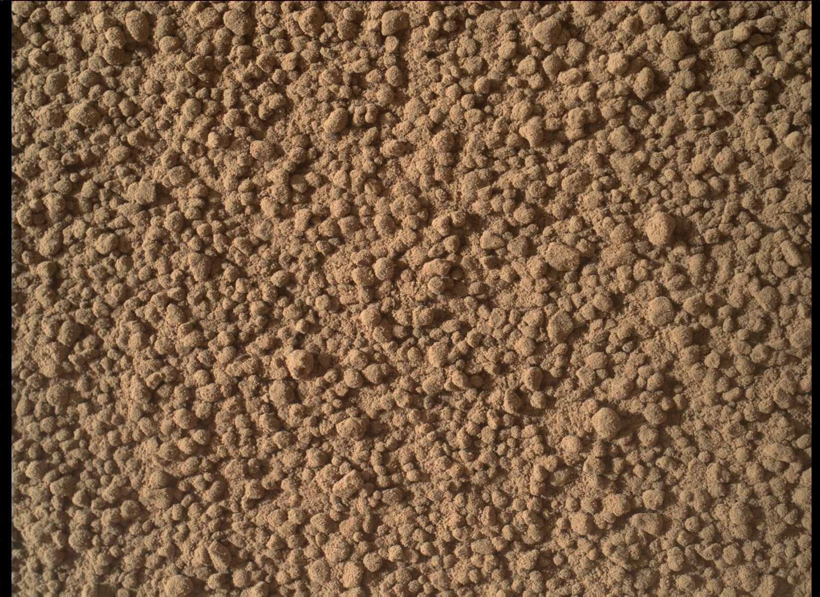
Coated Granules
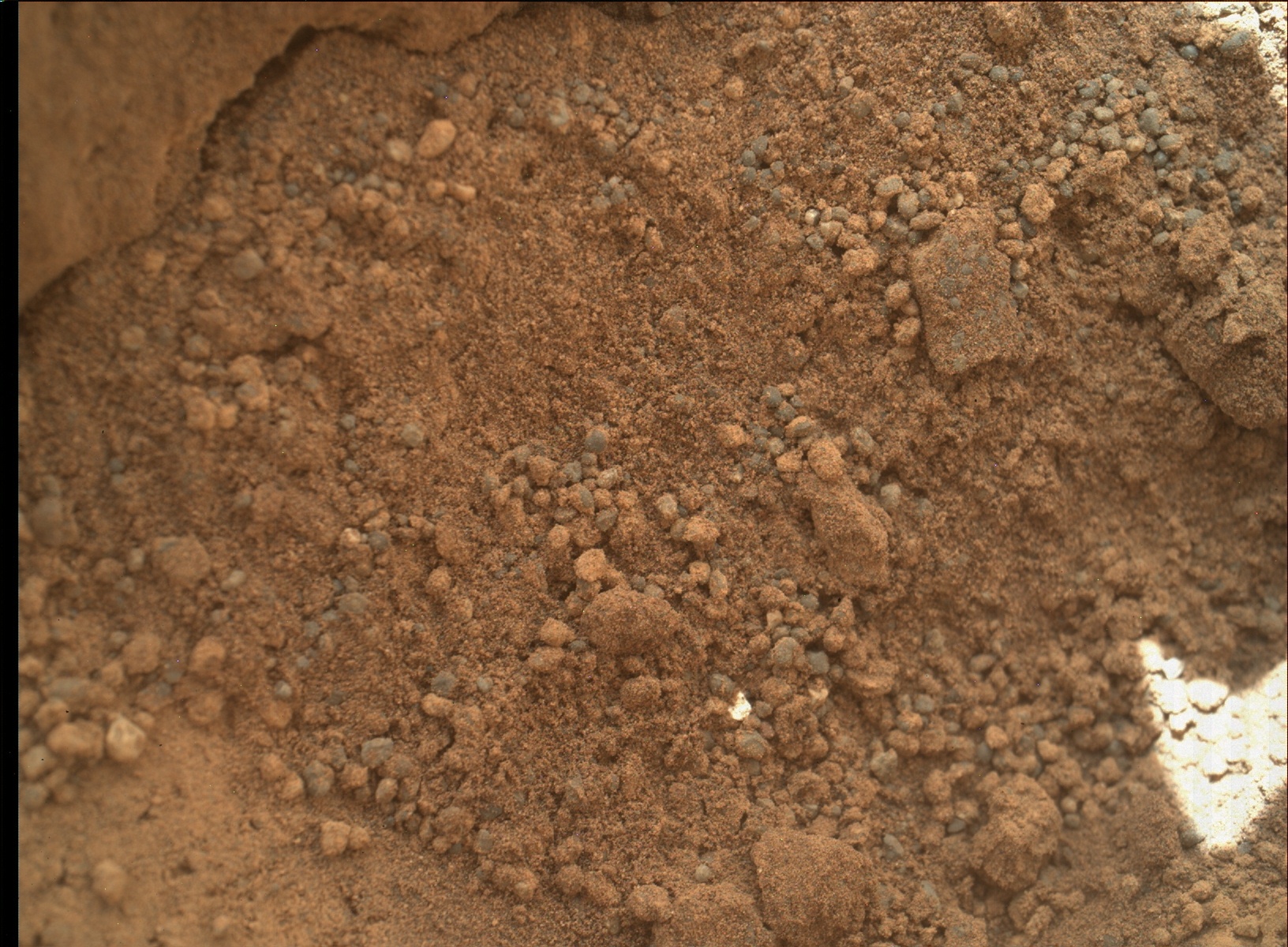 src: MSL Raw Images
This Sol 69 MAHLI image shows that the coating on the surface granules does not cover the entire granule. The interior of the granule looks like it might be a saltation particle. A possible explanation is that a layer of saltation particles collected at this location on top of a small sand drift and the fine powder coated them later. In a dust storm one would expect a light fine powder to be airborn the longest. Electrostatic or intermolecular forces might be what made them adhere together. On the surface light might play a role in breaking chemical bonds permitting new ones to form between adjacent particles. On Earth dampness helps things cling together.
Monday, October 15, 2012
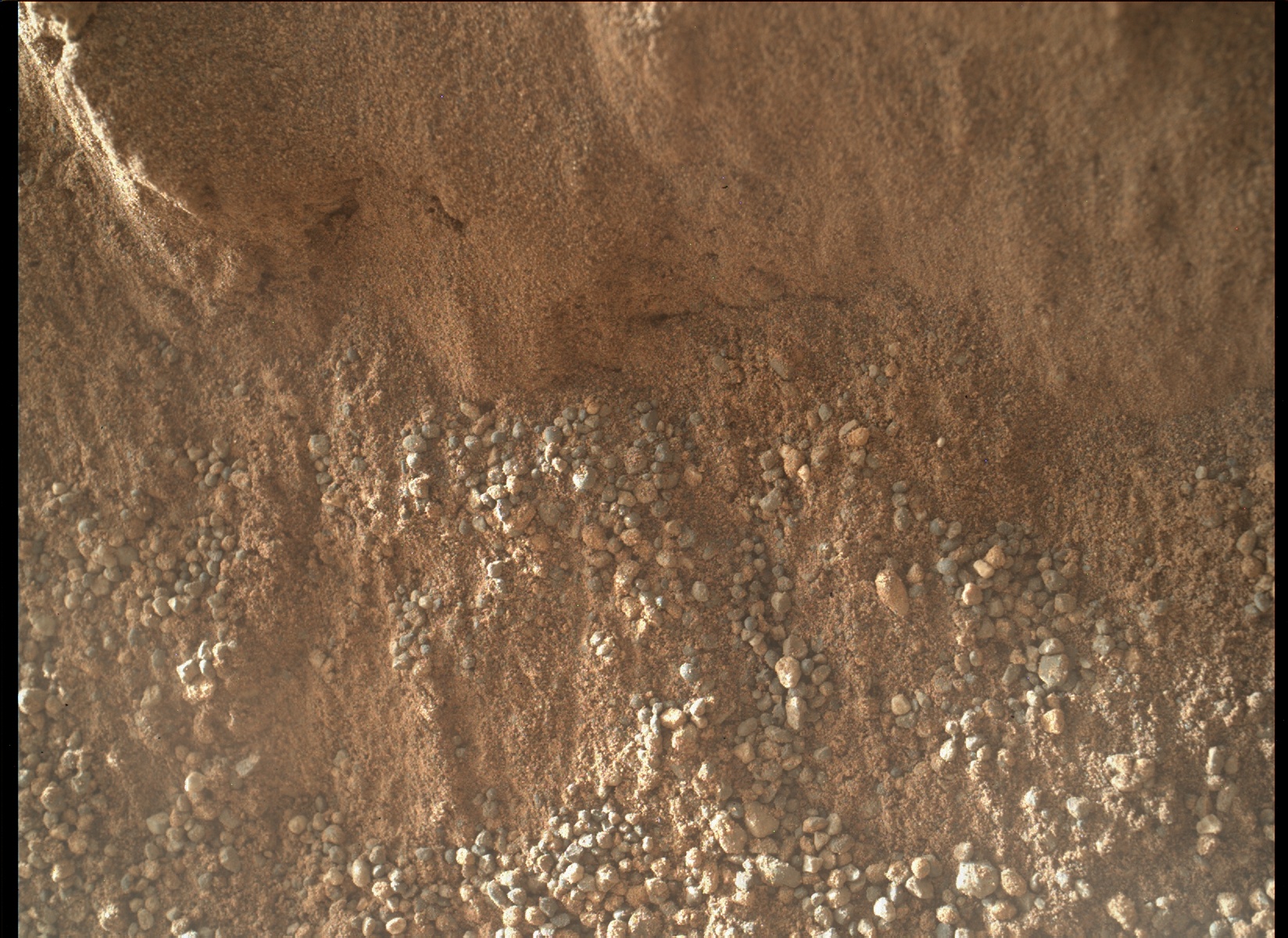
A Close-up of the Bright Object
 src: MSL multimedia
Curiosity managed to get a close-up of the mysterious bright object that was spotted in an Oct 7th image with the MAHLI hand imager. The small granules present appear to be of the same material as the sand or electrostatically coated.
Saturday, October 13, 2012
Galton - Selected Works on Heredity
Here is a list of selected works by Galton on the normal distribution and the heredity of physical traits along with their dates. They can be found at galton.org. Galton also made use of the error ellipse which is discussed in more detail in the appendices.
Typical Laws of Heredity (Feb 9, 1877)
Proceedings Royal Institution of Great Britain Volume 8
Regression towards mediocracy in hereditary stature p. 246 (June 9, 1885)
mentions J. Hamilton Dickson p. 255 (with figures)
Journal of the Anthropological Institute of Great Britain Volume 15
President's Address (1885)
Reports of the Meetings of the British Association for the Advancement of Science Volume 55
Family Likeness of Stature (January 21, 1886)
appendix by J. D. Hamilton Dickson (with figures)
Proceedings of the Royal Society of London Volume 40 p. 42
President's Address p. 489 (Annual General Meeting, January 26, 1886)
Journal of the Anthropological Institute of Great Britain Volume 15
Co-relations and their measurements (December 20, 1888)
Proceedings of the Royal Society of London Volume 45
Natural Inheritance 1894
Appendix B, Problems by J. D. Hamilton Dickson
reprinted from Proc. Royal Soc., No. 242, 1886, p. 63 (no figures)
Airy's Theory of Errors
The intellectual capital needed to calculate the means, moduli (scaling units) and quartiles in the last blog can be found in Airy, Theory of Errors of Observations (1875). The work appeared just before the start of Galton's series of publications on the normal distribution and heredity. Here is an index of the relevant sections.
§3 Law of probability, frequency of errors
mean error #24-6, p. 18f
squares of errors #27, p. 20
quartile #28-9, p. 22-3
§9, mean error, error of mean square #60-1, p. 45-8
§11, sum of weighted error #68, p.53
Airy's Theory of Errors also discusses solving for errors and "minimum squares" in §13, #87, p. 71f which are related to regression.
Galton's Use Of The Normal Distribution

Francis Galton wrote a number of papers in which he used the normal distribution in the study of human inheritance. The most mathematically complete paper appears to be Family Likeness in Stature, published in the Proceedings of the Royal Society of London, Volume 40, pages 42-73. The publication is dated January 21, 1886. The work seems to have been done with the assistance of J. D. Hamilton Dickson who was a tutor at St. Peter's College in Cambridge. Part of this paper is available in the collected papers at galton.org but part of the appendix and the tables at the end seem to be missing. The data for the inheritance of stature is from the Record of Family Faculties. I've been going over the mathematics used in the paper and have found a simple way to calculate Galton's measure of the deviation from the mean for the normal distributions. Column A in the table above contains a distribution of heights for the population in general and two sets of brothers. One can convert the frequencies in the tables to probilities by dividing by the sum of the columns. Multiplying the heights by the probabilities and adding gives the average height for each column. One can also calculate the standard deviation for each column and convert this to something like a scale height which can be used to determine the dimensionless parameter t. Galton uses the cumulative probability distribution analysis and quartile distances to characterize the spread of the distributions. For each distribution Galton found that the quartile distance qH = 1.7 inches. In general the height H = mH + t sH. An explanation of the terms can be found in the simplified Mathcad calculation seen below.

A better name for the scaling unit that Galton used might be "scale deviation". Computing the probabilites for one inch intervals and multiplying by the sum of each A column one gets these fits.


Supplemental (Oct 13): The calculation was intended to give a simple estimate of the scaling unit. One could get technical about the precise definition of standard deviation and the difference of estimated, expected and observed deviations. For one data point the observed deviation might be taken as zero but the standard deviation would be infinite.
Supplemental (Oct 15): The table above is from the Google eBook edition of the Proceedings of the Royal Society that was cited.
Thursday, October 11, 2012
2012 Nobel Prize for Literature
src: thenobelprize
Earlier today the 2012 Nobel Prize for Literature was awarded to the Chinese writer Mo Yan "who with hallucinatory realism merges folk tales, history and the contemporary".
Oct 11 Teleconference
src: Curiosity Cam - ustream
Today's MSL teleconference discussed the chemical composition of some of the rocks recently tested at Gale Crater with the main focus on Jake Matijevic. The images for the conference can be found on the NASA MSL telecon page and at the MSL Image Gallery. The rock Jake Matijevic was found to be have high concentrations of sodium, magnesium, aluminum and silicon and was a new type found on Mars. The closest rocks on Earth are found on the ocean floors. The process of their formation is referred to as alkalic. A melt such as that in a volcano can lose material through solidification which alters the composition of the melt leading to higher concentrations of some minerals. Water is also dissolved in the melt like cabon dioxide is dissolved in the liquid of a cola drink. The process was compared to the traditional method of producing cider. The cider is repeatedly frozen and the ice crystals are removed. The liquid remaining has a higher concentration of alcohol. Related geological processes are igneous differentiation, fractional crystalization and partial melting. It is difficult to deduce more about the conditions that led to the rock's formation since it is not known if it is part of a local rockbed or if it was relocated by meteor impact. The teleconference also discussed the first effort at decontamination of sample collection system and monitoring of the process.
Wednesday, October 10, 2012
2012 Nobel Prize for Chemistry
The Nobel Committee announced today that Robert J. Lefkowitz and Brian K. Kobilka are the recipients of the 2012 Nobel Prize for Chemistry "for studies of G-protein-coupled receptors." These receptors are located in the cell membrane and enable the cell to detect chemical messengers and respond to them. They are part of the mechanism which allows the cells of the body to communicate with each other.
Supplemental (Oct 11): The video of the announcement is now available at thenobelprize on YouTube.
Tuesday, October 9, 2012
2012 Nobel Prize for Physics
src: thenobelprize
The Nobel Committee announced today that the 2012 Nobel Prize for Physics goes to Serge Haroche and David J. Wineland "for ground-breaking experimental methods that enable measuring and manipulation of individual quantum systems." Both researchers have done work on Quantum Optics which is concerned with the interaction between light and matter. Some articles on their work:
Monday, October 8, 2012
2012 Nobel Prize for Physiology or Medicine
src: thenobelprize
Today the Nobel Committee announced the recipients for the 2012 Nobel prize for Physiology or Medicine. They are Sir John B. Gurdon and Shinya Yamanaka. The prize was awarded for showing that genetic material from mature cells could be transferred into an egg subsequently developed into complete organisms and that this could also accomplish by reprogramming individual cells.
Curiosity's First Scoopful of Mars
On Sol 61 Curiosity captured a MastCam video of the scoop vibrating a sample of from one of the drifts at Rocknest. Here are some more images.

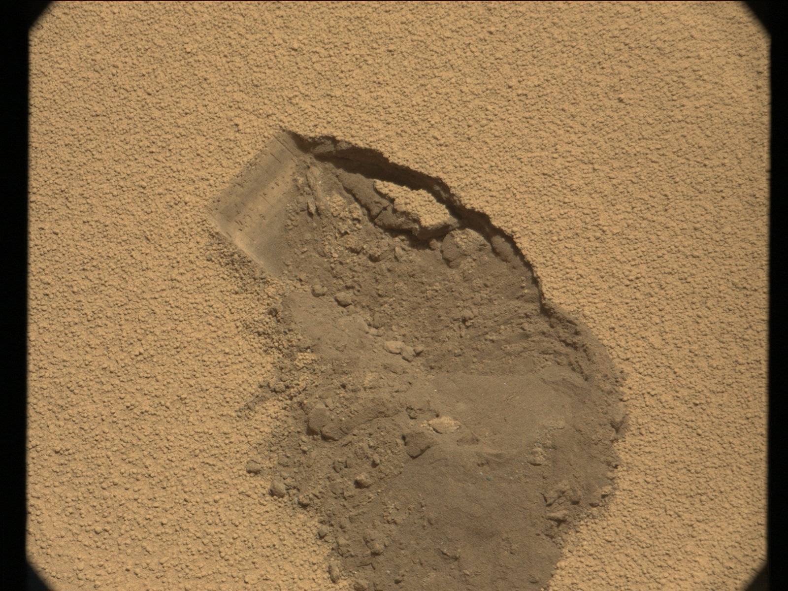 src: MSL Raw Images
Friday, October 5, 2012
Oct 4 Teleconference & Close-up Images Of A "Ripple"
The MSL Oct 4 telecon dwelt on the plans for the next couple of weeks at the Rocknest site to scoop material from a "sandbox" there. The sampling system first needs to be purged and cleaned of contaminants by doing a number of trial runs through it. The process will be more closely monitored initially to verify the proper functioning of the system. The caption for the conference image with the wheel impression on one of the drifts refers to it as a ripple. The Sol 58 MAHLI close-ups shows that the ripples consist of a crusty coarse grain layer resting on top of a more sandy one. The coarser grains may be saltation particles.
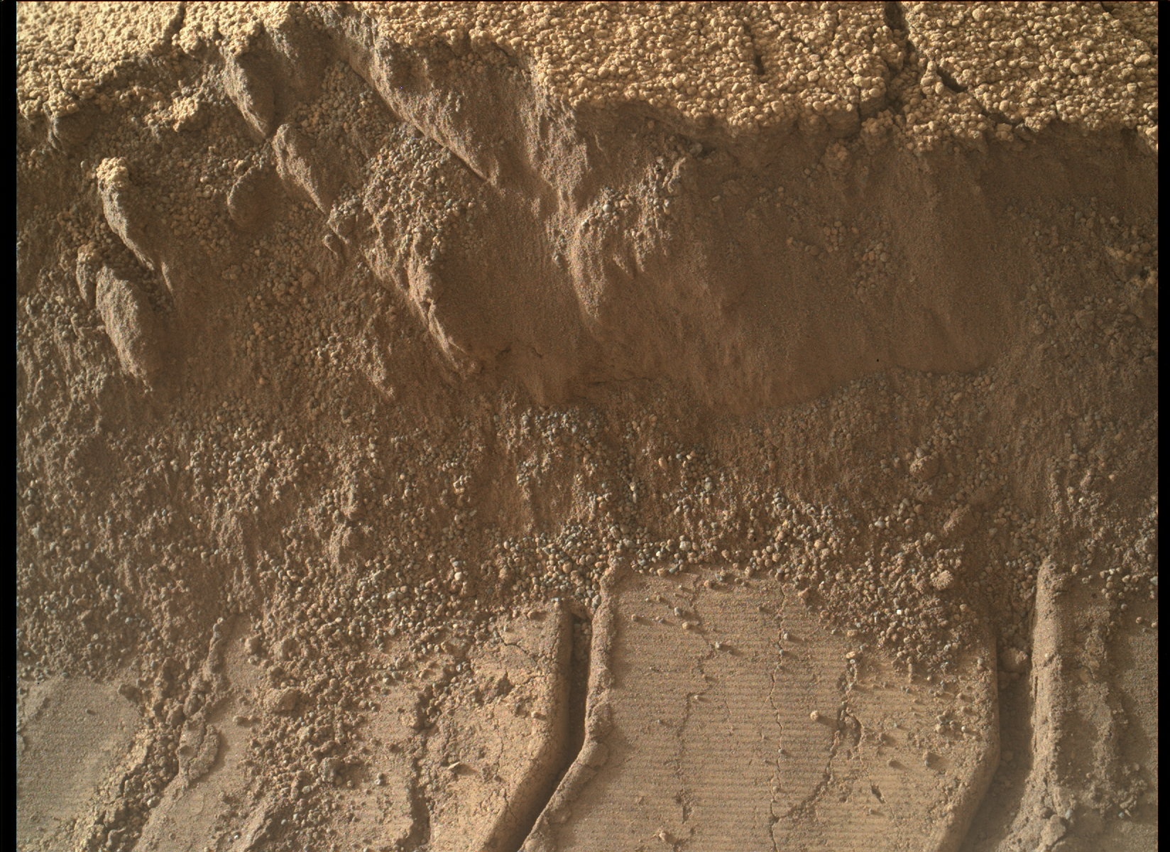
Supplemental (Oct 5): A zastryga, Russian заструга, is an inanimate object. It is fixed in place. There are other things like bow waves that are relatively fixed in place that fit in a more general class with similar attributes. Tags may be useful in identifying them.
Subscribe to:
Posts (Atom)