 On multiplying these numbers by the number 11 we find that the frequency corresponding to the note A is exactly 440 cycles per second. A440 is now the standard frequency for the musical scale. Helmhotz arrives at the same set of numbers in On the Sensation of Tone and attributes the scale to Scheibler.
Thursday, December 29, 2011
Scheibler's Musical Scale
Helmholtz did a calculation of the frequencies of the musical scale. Like him we can start out with the ratios of Ptolemy's scale. Using the numerators, n, and denominators, d, below the ratios are n/d. If we want to adjust these numbers so the all the denominators are the same, the smallest denominator that will accomplish this task is D = 24. The corresponding numerators are N = 24, 27, 30, 32, 36, 40, 45, 48. These numbers are the harmonics of a fundamental frequency whose value is 1/24th that of Middle C and are part of a harmonic series.
 On multiplying these numbers by the number 11 we find that the frequency corresponding to the note A is exactly 440 cycles per second. A440 is now the standard frequency for the musical scale. Helmhotz arrives at the same set of numbers in On the Sensation of Tone and attributes the scale to Scheibler.
On multiplying these numbers by the number 11 we find that the frequency corresponding to the note A is exactly 440 cycles per second. A440 is now the standard frequency for the musical scale. Helmhotz arrives at the same set of numbers in On the Sensation of Tone and attributes the scale to Scheibler.
The Beat of a Different Drummer?
For Christmas I got a set of tuning forks from scientificsonline.com.

The pitches marked on the forks are,
C: 256, D: 288, E: 320, F:341.3, G: 384, A: 426.6, B: 480, C:512
which are not the usual pitches used in music. The label on the box doesn't help much by way of an explanation of the difference.

The notes indicate that it is a diatonic scale and the proportions (fork pitch/C256) are as follows,
1, 9/8, 5/4, 4/3, 3/2, 5/3, 15/8, 2
indicating a Ptolemaic diatonic scale. One may ask, "Why is this particular scale is used?" It presented a bit of a puzzle and further study was indicated.
I consulted Rayleigh's The Theory of Sound and found the C256 "is usually adopted by physicists and acoustical instrument makers, and has the advantage of simplicity." But he says nothing of its origin. Helmholtz in On the Sensations of Tone is not much more helpful. He does refer to "The theorectical English pitch, c' = 256" which indicates an English origin. Through a Google book search I came across Ellis' History of Musical Pitch which mentions C512 and a report by the Society of Arts. Another book search led to an entry in the Journal of the Society of Arts, Jun 10, 1859 which discusses the need for a "uniform pitch or diapason." C512 was favored by Mr. Hullah. The signatures there indicate that members of the Royal Society were present. One also get the impression the C512 scale predates this discussion. A paper, The origin of the tuning fork, that I found at the National Institutes of Health indicates that John Shore and Handel used this scale.
So this may be a partial explanation for why this particular scale is used by the scientific community.

The pitches marked on the forks are,
which are not the usual pitches used in music. The label on the box doesn't help much by way of an explanation of the difference.

The notes indicate that it is a diatonic scale and the proportions (fork pitch/C256) are as follows,
indicating a Ptolemaic diatonic scale. One may ask, "Why is this particular scale is used?" It presented a bit of a puzzle and further study was indicated.
I consulted Rayleigh's The Theory of Sound and found the C256 "is usually adopted by physicists and acoustical instrument makers, and has the advantage of simplicity." But he says nothing of its origin. Helmholtz in On the Sensations of Tone is not much more helpful. He does refer to "The theorectical English pitch, c' = 256" which indicates an English origin. Through a Google book search I came across Ellis' History of Musical Pitch which mentions C512 and a report by the Society of Arts. Another book search led to an entry in the Journal of the Society of Arts, Jun 10, 1859 which discusses the need for a "uniform pitch or diapason." C512 was favored by Mr. Hullah. The signatures there indicate that members of the Royal Society were present. One also get the impression the C512 scale predates this discussion. A paper, The origin of the tuning fork, that I found at the National Institutes of Health indicates that John Shore and Handel used this scale.
So this may be a partial explanation for why this particular scale is used by the scientific community.
Monday, December 26, 2011
Founders Tree
In Humboldt Redwoods State Park near Weott, CA along an old route of Hwy 101, also known as The Avenue of the Giants, is Founders Grove in which one can find one of the tallest living trees in the world. It's known as The Founders Tree and is dedicated to the founders of the Save-The-Redwoods League. It is 346.1 feet or 111.0 meters tall.
Founders Tree
It's not the tallest tree in the park. That title is claimed by Stratosphere Giant. The tallest redwood currently known is Hyperion in Redwood National and State Parks.
Supplemental (Dec 27): The Founders Tree coordinates on a
USGS topographic map (CA Weott 102418 1969 24000 geo)
are 40° 21.121'N, 123° 55.426'W.
Friday, December 23, 2011
Dark Winter Nights
Some of you may have noticed how dark it is at night these days. One reason is that the Winter Solstice was on Dec 22 at 5:30:00 UT. The US Naval Observatory's Multiyear Almanac gives the times of the Winter Solstice for when the Sun crosses Right Ascension 18 hours. Another reason is that the New Moon also occurs this week on Christmas Eve at 18:06 UT. I used the Almanac to compute the angular distance between the New Moon and the Sun at the time of the Winter Equinox to see how often they occur together between the years 2000 and 2050.

The plot above shows that this is a rather rare event astronomically but in 2014 they will come rather close together, less than 1.5° in RA apart. The probability of this happening is about once in 240 years. The average number of days in a month is the Moon's synodic period of 29.5 days. So the probability that the New Moon will occur on the same day as the Winter Solstice is about once every 30 years.

The plot above shows that this is a rather rare event astronomically but in 2014 they will come rather close together, less than 1.5° in RA apart. The probability of this happening is about once in 240 years. The average number of days in a month is the Moon's synodic period of 29.5 days. So the probability that the New Moon will occur on the same day as the Winter Solstice is about once every 30 years.
Tuesday, December 20, 2011
Greenland Geological Record Atypical?
When looking at the geological record for a given locality we have to look at extraneous factors factors which might influence conditions. There is a Croll quote from Lyell's Antiquity of Man referring to a warmer Greenland in the past and evidence of plant life there. However, Greenland may be atypical because of the presence of "numerous hot springs" on Disko Island, the location mentioned. This may be a contributing factor for Sequoia langsdorfii being able to grow at such a high latitude.
It would be interesting to see what radiocarbon or some other form of radiometric dating would tell us about the age of the fossils found. One has to be careful about the assumptions one makes when extrapolating the proxy temperature records and not read too much into them. Paleontology and the fossil record may provide some additional information over a longer span of time.
It would be interesting to see what radiocarbon or some other form of radiometric dating would tell us about the age of the fossils found. One has to be careful about the assumptions one makes when extrapolating the proxy temperature records and not read too much into them. Paleontology and the fossil record may provide some additional information over a longer span of time.
Monday, December 19, 2011
Ancient Sequoia
Both Croll and Lyell discuss the change in climate over time for a given locality. An example is the Sequoia which is now only found in California and Oregon on the west coast of the United States. The fossil species Sequoia langsdorfii is nearly indistinguishable from the modern species Sequoia sempervirens.
Some S. langsdorfii links are:
Fossil Record of the Redwoods - NPS
On the Change of the Obliquity - Croll
Elements of Geology - Lyell
Some S. langsdorfii links are:
Fossil Record of the Redwoods - NPS
On the Change of the Obliquity - Croll
Elements of Geology - Lyell
Friday, December 16, 2011
Croll's Climate Change papers, 1864-7
It can be a little difficult to keep track of Croll's papers on climate change spread out over the years from 1864 to 1867 in Philosophical Magazine. A list might prove useful.
Aug 1864, p. 121, On the Physical Cause of the Change of Climate during Geological Epochs
Jan 1866, p. 26, On the Excentricity of the Earth's Orbit
Apr 1866, p. 301, On the Physical Cause of the Submergence and Emergence of the Land during the Glacial Epoch
Feb 1867, p. 119, On the Excentricity of the Earth's Orbit, and its Physical Relations to the Glacial Epoch
Jun 1867, p. 426, On the Change in the Obliquity of the Ecliptic, its Influence on the Climate of the Polar Regions and on the Level of the Sea
These papers can be found elsewhere and much of the content is reproduced in Croll's first book.
Thursday, December 15, 2011
Another Croll Climate Change Paper From 1867
Earlier today I found another climate change paper by James Croll, On the Eccentricity of the Earth's Orbit, and its Physical Relations to the Glacial Epoch, published in Philisophical Magazine, Feb., 1867. It appears to have be written about the same time as the Geological Society of Glasgow paper on the change in the obliquity. The obliquity paper is rather interesting especially the part about 25 ft and 40 ft beaches at 11,700 years ago and 60,000 years ago respectively. Forests below the present sea level that alternated with mud flats point to rather large changes in sea level possibly due to the melting of a mile of the Antartic ice sheet and a shift of the Earth's center of gravity northward about 8 ft. The implication seems to be that the Arctic Ocean will rise somewhat when aphelion and the winter solstice coincide.
Wednesday, December 14, 2011
Croll's 1864 Paper on Climate Change
James Croll's first paper on climate change, On the Physical Cause of Climate Change during Geological Epochs, was published in 1864 in Philosophical Magazine, Vol 28. In it he starts out by reviewing earlier discussions of climate change and proposes an alternative theory. He notes that in past ages there were alternating periods of warm and cold which could be deduced from the species of sea shells that were present in the oceans around England. Glaciers and icebergs transported broken rock which ended up as breccias in the seas. A warm period was responsible for the coal formations in England. He suggests that the cold period may have been due to an absence of the Gulf Stream at that time. There is a discussion of trade winds and ocean currents. He proceeds to a discussion of Leverrier's work of the variation of the eccentricity of the Earth's orbit and the effect of the Earth's precession in alternating the temperature of the northern and southern hemispheres. Finally he correlates these temperature changes with the warm and cold periods in the two hemispheres.
Supplemental (Dec 14): Another paper, On the Change in the Obliquity of the Ecliptic, was published in the Transactions of the Geological Society of Glasgow in 1866.
Supplemental (Dec 14): Another paper, On the Change in the Obliquity of the Ecliptic, was published in the Transactions of the Geological Society of Glasgow in 1866.
Friday, December 9, 2011
Croll on the Heating Power of Ocean Currents
Capter 2 of Croll's Climate and Time in their Geological Relations uses the Atlantic Gulf Stream to show the heating power of ocean currents. The Gulf Stream flows along the eastern coast of North America from the Caribbean to northern Europe. The heat it carries with helps moderate the climate of northern Europe. His estimate of the amount of heat transported might be a little diffucult to follow and some illumination would probably help. He starts out with a simple channel-like model of the Gulf Stream.
 His units are somewhat outdated. The foot pound is the amount of energy required to lift a pound mass 1 foot against the force of gravity. The rate of flow of sea water in the channel is Q = depth * width * speed of the flow. To compute the heat capacity of a cubic foot of sea water we need to know the density of sea water and its specific heat capacity. Croll uses the density of ordinary water and assumes we know the density of sea water1. Multiplying these values by the change in temperature gives the heat per unit volume transported away from the Caribbean. The total heat transported per day is the heat per unit volume times the volume rate of flow. Doing the math gives us the numbers cited by Croll.
 Croll also makes an estimate of the rate of solar heating or the amount of heat recieved by a unit of area in a unit of time for a point on the equator at one of the equinoxes. He starts out with a value close to Pouillet's for the rate of heating at the top of the atmosphere and uses an estimate that 22% is stopped by the atmosphere. Again we get the value cited for the heat flux at the surface.
 Croll notes that for the current orbit and orientation of the Earth the southern hemisphere gets more heating than the northern hemisphere which experiences milder conditions. Since the northern hemisphere is colder there is some heat transport across the equator. If we look at the ocean currents in the Atlantic near the equator we see that there is a current from the Tropics off the west coast of Africa along the equator that transfers to the east coast of South America and up into the Caribbean some of which ends up in the Gulf Stream.
Supplemental (Dec 10): 1The value used for the volume heat capacity appears to be the one used by Croll. I used the specific heat capacity for sea water at a slightly higher temperature (20°C or 68°F) and the density of fresh water. The error seem to be negligible. The specific heat capacity for sea water is slightly less than that of fresh water since there are fewer molecules for a given weight due to the presence of the dissolved salts. The salts also increase the density of sea water slightly to 1.025 gm/cm3.
Wednesday, November 30, 2011
A Short Walk Through Some 19th Century Science
These links are from a somewhat random online stroll through some 19th Century scientific literature that I made this Tuesday.
On the Relative Motion of the Earth and the Luminiferous Ether, Albert A. Michelson, American Journal of Science, Nov, 1887
The relative motion of the Earth and the Luminiferous ether, Albert A. Michelson, American Journal of Science, Aug, 1881
A Contribution to Croll's Theory of Secular Climatal Changes, W.J. McGee, American Journal of Science, Dec, 1881
William John McGee - Wikipedia
James Croll - Wikipedia
James Croll in Context - jfleming, ICHM
Meteorology - Wikipedia
Letter on the change in the perihelion of Mercury - LeVerrier, Comptes Rendus, Sep, 1859
Charles Lyell - Wikipedia
Principles of Geology, Vol. I, Chapter XIII, Charles Lyell
Supplemental (Wed):
Joseph Adhemar - Wikipedia (very 2012)
Climate and Time in their Geological Relations, James Croll, 1875
Discussions on Climate and Cosmology, James Croll, 1885
Révolutions de la mer, Joseph Adhémar, 1842 (tipping point?)
Thursday, November 24, 2011
Relativity and Sun Grazing Orbits
One reason why I said that Relativity is juvenile is the postulate that the speed of light is a constant. Michaelson and Morley got a null result for measuring the effect of the Earth's motion on the speed. The changes throughout the year were less than the uncertainty of the error in the measurements. So to a high degree of approximation the speed of light for the Earth is a constant. Raising this to the level of an axiom though goes beyond the supporting evidence. It works just as well as an approximation as an axiom. Einstein may have claimed a little too much but the Theory of Relativity does make a good working hypothesis.
For a circular Sun grazing orbit the orbital speed is about 440 km/s and fraction of the speed of light β = v/c = 0.0015. For a highly elliptical Sun grazing orbit the perihelion speed is about 620 km/s and β = 0.0021. So the elliptical orbit is the worse case for bodies orbiting the Sun and the resulting increase in mass is only about 1 part in 500,000. Relativity only has a minor effect on an orbiting body but errors that accumulate over centuries are noticible.
For a circular Sun grazing orbit the orbital speed is about 440 km/s and fraction of the speed of light β = v/c = 0.0015. For a highly elliptical Sun grazing orbit the perihelion speed is about 620 km/s and β = 0.0021. So the elliptical orbit is the worse case for bodies orbiting the Sun and the resulting increase in mass is only about 1 part in 500,000. Relativity only has a minor effect on an orbiting body but errors that accumulate over centuries are noticible.
Wednesday, November 23, 2011
The Mature vs Juvenile World Views
While studying the Gaussian gravitational constant and its constant function I found that the function and the elliptical orbit remain unchanged in General Relativity's rotating (precessing) orbital plane. The equation for the orbit has an extra term, 3mu2 (u = 1/r), in GR. This shouldn't be surprising since motion in Relativity confuses space and time a little. The term is small compared to other terms in the equation of the motion and the solution for planetary orbits found in Eddington's The Mathematical Theory of Relativity used the classical orbit as a first approximation to derive a relativistic correction. Eddington also makes an assumption that the mass is constant since p = h2/μ is dependent on mass which relativistically varies with the speed at which a body is moving. For highly elliptical orbits the speed at perihelion near the Sun is much greater than at aphelion, the most distant point in the orbit, and we may expect the approximations made to break down a little.
But Relativity makes some assumptions like the speed of light being a constant which can be considered an approximation too. The results of Relativity are based on deduction which is more accurate than induction and it draws heavily on classical results such as the agreement of the form of the gravitational potential with classical theory. For a two-body problem in GR one has to work with two world lines and coupling their motion assumes a rigid rotor. This like all other constraints restricts the solution to the problem. The check on results is a correspondence principle which says that the results of GR should agree with classical results for low velocities and small masses but one is free to speculate about initial the possible changes that one can make.
The dependence of the results of Relativity on classical physics makes it appear somewhat juvenile. It doesn't appear to be able to stand on its own as one would expect of a more mature theory. The initial assumptions that one can make have a lot of room for error that the correspondence with the classical limit can't narrow down. The same is true for Quantum Mechanics which has a similar approach to the problem and has to deal with uncertainties of its own. In QM one seems to be solving for theories to fit the facts. The results can sometimes be confusing and contradictory which the Schrodinger's cat thought experiment tried to point out. In the quantum world one can never have a clear picture of what is happening and one tends lose track of events.
One's comprehension may be limited but that doesn't mean that theory itself is bounded by one's limits. Are we being held back by a juvenile world view or is there still room for change. We probably shouldn't forget that change comes from within. And additionally we need to narrow down what is "good conduct" in Science. That might be a sign of movement towards a more mature approach.
Wednesday, November 16, 2011
The Gaussian Gravitational Constant
In Theoria Motus (1809) Gauss gave a formula which he stated was a constant for all bodies orbiting the Sun. This quantity, k, has come to be known as the Gaussian gravitational constant. The formula Gauss gives is,
 ΔA/Δt, the areal velocity, is the area ΔA swept out by the body's radius in time Δt, and is a constant for a single body according to Kepler's 2nd law. p is the parameter in the formula for the elliptical orbit of a body and m is the body's mass given in solar masses. This is based on a two-body solution for an orbit about the Sun and gravitational perturbations by other bodies are ignored. In the two-body problem one can replace the mass of a body with its reduced mass. M presumably represents the mass of the Sun.
The Moon and the Earth are gravitationally bound so their motion is coupled and we would have to use the sum of their masses in the formula to get it work properly. But does M truly represents the mass of the Sun if we have to treat gravitationally bound together or is this only an approximation? The other planets are gravitationally bound to the Sun so in treating this as a two-body problem we are splitting the solar system into two parts, the Earth-Moon system and the rest of the Solar System with the total mass being M'(m1 + m2) where m1 is the mass fraction of the other bodies in the Solar System and m2 is the mass fraction of the Earth-Moon system. Instead of 1+m on the left we would have m1 + m2 = 1 and a mass term would not be present in the formula. Even though the fractions were different for each body and the "Sun" the sum of the two masses would have the same value, M'. Gauss' formula would then be approximately correct since the mass of Jupiter is about one thousandth that of the Sun. The formula that Gauss gave may work better for single orbits but over long periods of time one may notice a discrepancy with the perturbations of the orbits being a complication.
Tuesday, November 8, 2011
Loading Orbital Elements in Distant Suns
Loading orbital elements into astronomy programs can be challenging at times. I have an older one, Distant Suns, that works quite well but is in need of an update. The HORIZONS ephemeris provides the osculating orbital elements for an object. This provides enough information to specify the orbit if the definitions are known. The process of loading the elements for 2005 yu55 into Distant Suns is shown below and the program shows the its location at the time of closest approach to the Earth. The time shown at the bottom of the image is UT.

click for clearer view
The HORIZONS User Manual gives the following definitions for the elements,

Not all of these elements are needed to specify an orbit. For example the ascending node can be used instead of the longitude of perihelion since the latter is just the sum of the ascending node and the argument of perihelion. Another drop down menu would have been more useful. This method was used for the choice between periapsis and the semi-major axis which specify the size of the orbit.
Monday, November 7, 2011
Tracking 2005 YU55
2055 YU55 is rapidly approaching the Earth. The closest approach is about 0.0021374 AU Nov 8 23:30 UT. It is very faint being a 12th magnitude object so a good telescope is required to see it.

One can follow its approach using the JPL Small-Body Database Browser. This site requires Java to view the plot of the orbit. Center on the Earth and zoom in to follow the relative motion. One can also generate an ephemeris for 2005 YU55 using links on the page.
The conditions for the fly-by favor Europe but after sunset on the US east coast one might be able to track it as it moves towards the Moon. The New Moon is on Nov 10 and may complicate viewing.
Friday, November 4, 2011
Asteroid 2005 YU55 Close Encounter Nov 8, 2011
2005 YU55, a 400 meter asteroid, will pass within the distance of the Moon of the Earth on Nov 8, 2011. It will pass within 0.85 lunar radii (325,000 km) of the Earth and 239,000 km of the Moon. It is considered a Potentially Hazardous Object because of the proximity of its orbit to that of the Earth's and the chance of an impact although that is not likely to happen in the near future.
Thursday, October 13, 2011
Angular Separation as the Distance Correlation
One can use other numbers besides powers of 2 for the number system of the random-number generator. Here 54 = 625 is the number of objects that are chosen from. A sample of 9001 numbers was generated. The generator seems to work better with larger numbers which is why 54 was used. The resulting numbers can be converted into their base 5 representation and the four resulting base 5 numbers could be used to represent a part of a sample drawn from 5 objects.

Instead of the autocorrelation of the string of numbers with shifted versions of itself, a dot product was taken and the resulting anglar separation was used as the distance correlation. The "demons" are still present and occur at the midpoint of the sample.

The average projection of the unit vectors of one member of the sample onto another is 3/4 so the average normal would be about √7/4. This corresponds to an angular separation of 41.41°.

As can be seen, the distribution of the angular separations agrees fairly well with the expected mean. One might expect some variation from it if the initial (reference) "direction" is atypical and therefore an outlier.
The simplest definition of a distance correlation for generator strings of the same length would probably be the angle between their unit vectors or,
dcorr(e1,e2) = acos(e1·e2).
Thursday, October 6, 2011
Getting Past the Demons
The problems that were encountered with the random-number generator resulted from trying to simplify it for the last post. I had been using larger numbers at first and reduction past a certain point started introducing more regularity in the output of the generator. If one wants the generator to produce numbers varying from 0 to n-1, the choice for α and μ are related by the formulas below.

The "demons" disappear in this version of the generator. The mirror symmetry problem in the output seems to have moved elsewhere. The simpler version of the generator raises the question of what we mean by statistical independence? Are mirror images of sequences allowed? If we treat sequences of numbers as the ordered numbers found in a vectors then two sequences are related if they are multiples of each other or reflected versions of each other. The vector B = mA which results by multiplying the vector A by m is related to A. The vector (y,z,x) is a permutation of the elements of (x,y,z) and so also related. But we have to allow these sequences since they are valid outputs for the generator. The question is really one of the frequency with which these sets of numbers occur. One has to look at a set of output sequences and determine whether or not the set is statistically likely. In creating a set of sequences we can compare each new entry with the existing set and reject it if it is too closely related.
Correlation was used to compare sequences of numbers. It tells us how well two sets of numbers are aligned. If they are too closely aligned it raises doubts about their statistical independence.
A reference for this random-number generator is Hamming, R.W., Numerical Methods for Scientists and Engineers, pp. 137-42.
Supplemental: The random-number generator's mechanism appears to be closer to that of the urn problem than that of shuffling. Shuffling permutes the order of the cards in a deck. Picking a card at random is an urn problem.
Tuesday, October 4, 2011
A Random-Number Generator
There are times when a programmer needs to pick a number at random and the random-number generator was introduce to fill the need. The trick used is to multiply two numbers together and select a central string of digits. Below is a simple random-number generator. mod is the modulo function which gives the remainder that results when one number is divided by another.

This generator produces numbers between 0 and 1023 inclusive. A plot of the first 8192 numbers that it produces is shown below. The pattern appears to be quite random.

To evaluate a random-number generator one can count the number of times some number recurs in a sample and plot the freqency of no occurances of a number, just one occurance, two, three, etc versus the number of occurances. The generator above yields a Poisson distribution.

To see how internally random the sequence of numbers is one can compare it with a shifted version of itself using the correlation function. This is known as autocorrelation. Correlation varies between -1 and 1. The correlations between the shifted sets of numbers is quite small.

The observed values for the correlations vary between -0.05 and 0.05 and they appear to be distributed according to a normal distribution.

The sequence of numbers does indeed appear to be random. But if one looks closely at the plot of the correlations one can see that the left and right sides are mirror images of each other. So random-number generators are only useful up to a given point and can repeat after some period.

Close-ups of the center of the correlation plot confirms that demons are likely to be present in random-number generators. One nice thing about them though is that the results are reproducible.
Wednesday, September 28, 2011
UARS Reentry Location
The NASA UARS assessment says that the reentry location is 14.1°S, 170.2°W.
UARS Reentry reports that UARS reentered the earth's atmosphere at 10.65°S, 168.0°W.
Both locations are near the American Samoa.

The red line marks NASA's limits for the location of the debris field.
UARS Reentry reports that UARS reentered the earth's atmosphere at 10.65°S, 168.0°W.
Both locations are near the American Samoa.

The red line marks NASA's limits for the location of the debris field.
Tuesday, September 27, 2011
Lift and Drag for Extremely High Altitudes
Using a simplified model we can derive the formulas for lift and drag for a plate at high altitudes (above that of the mesosphere). The initial assumptions are that the particles present act independently, that in the reference frame of the plate the angle of incidence equals the angle of reflection for a particle bouncing off the plate and that its speed before and after are the same in this frame. The angle of the plate to the direction of motion is α. The direction of the particle after the collision in the frame of the plate is "e".

The initial and final conditions for the collision are as follows from which we can find the initial and final total momentum and kinetic energies.

Equating the momentum and kinetic energy before and after the collision we can determine the work done as the plate moves and the force acting on it.

One can see here that the values are reduced for particles deflected sideways from the those for a plate perpendicular to the direction of its motion. Completing the derivation we find the formulas for the lift and drag. CL and CD are the lift and drag coefficients.

The values for the coefficients are larger than normally encountered. At extremely high altitude the gases present have large separations between them so they have no viscosity and no cohesion. Intermolecular forces do not play a role.
For a more accurate calculation one might try scattering theory. For orbital speeds we can't assume that all collisions are perfectly elastic.
Edit (27 Sept): Changed the subscript of the resultant coefficient from N to R. The resultant is normal to the plate in its frame of reference. I was influenced by the some history in choosing the symbol for it (see Anderson's A History of Aerodynamics pages 104 & 169).
Thursday, September 22, 2011
Drag Force For Non-interacting Particles
For an extremely rarefied atmosphere we can assume that its particles do not interact with each other and that the collisions with the moving spacecraft are independent. To simplify the problem we represent the spacecraft by a flat plate of mass M perpendicular to the direction of motion and moving with a speed V. Let an individual particle of mass m be initially at rest. From the point of view of the plate the particle initially moves toward it with speed V and after the collision it will move away from it with speed V if no energy is lost in the collision and the mass of the particle is much less than the mass of the plate. To get the view from the perspective of the surrounding atmosphere we have to add the speed of the plate to these values for the speeds of the particle and we get v = 0 before the collision and v = 2V after. If n is the number density of the atmosphere the work, ΔW, done by the plate on N particles as it moves through a distance Δx and the drag force, D, are determined as follows.

The pressure, D/A, is known as ram pressure. If the particles are sent off sideways by the collision the drag force and the pressure are reduced. The corrective factor depends on the geometry an object. If a spacecraft with a flat forward surface is not perpendicular to the direction of motion but at an angle the resulting lateral force can produce lift and cause the spacecraft to skip off the atmosphere.

The pressure, D/A, is known as ram pressure. If the particles are sent off sideways by the collision the drag force and the pressure are reduced. The corrective factor depends on the geometry an object. If a spacecraft with a flat forward surface is not perpendicular to the direction of motion but at an angle the resulting lateral force can produce lift and cause the spacecraft to skip off the atmosphere.
Wednesday, September 21, 2011
Atmospheric Reentry And Its Effects
At what altitude does the density of the atmosphere become significant and contribute to reentry? To answer this question we can look at atmospheric models such as the US Standard Atmosphere or the International Standard Atmosphere. NRLMSISE-00 models the upper atmosphere and indicates that its density at 100 km about 10-10 g/cm3 decreasing rapidly with increasing altitude.
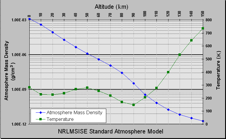
The ideal gas law tells us that pressure, temperature and density are related by the formula P=ρRT/M. The number density, number of molecules per unit volume, is n=ρ/m where m is the mass of the molecular component. Since the mass of a molecule is quite small the number of particles can still be quite large. This accounts for the atmospheric drag on a satellite. There is still some drag at higher altitudes.
When a meteor or satellite enters the atmosphere at high speeds a shock wave forms in front of it compressing the atmosphere. As the atmosphere is compressed it heats up and becomes luminous. Energy is released in the form of light by the Stefan-Boltzmann law. The pressure from the shock wave acting on the satellite slows it down and drops it out of orbit. Given enough time the satellite will reach a terminal velocity in the atmosphere which is much lower than its orbital velocity.
Meteors and spacecraft can skip off the atmosphere. During meteor showers the bolides pass through the upper atmosphere and can skip off it.
Tuesday, September 20, 2011
UARS Is Definitely Descending From Orbit
UARS is predicted to make its reentry sometime this weekend possibly late Friday evening or early Saturday morning depending on one's time zone. I have been studying the changes in the satellite's orbital elements and did a polynomial fit to the UARS's perigee as a function of the UTC day of the year. The plot below is the "altitude" as defined by the difference between UARS's perigee and the Earth's equatorial radius. The eccentricity is also decreasing which means that the orbit is becoming more circular.

It is predicted that UARS will reenter off the east coast of Africa but the exact location and time are somewhat uncertain. UARS probably has its greatest interaction with the Earth's upper atmosphere near the Equator because of the equatorial bulge and greater height of the atmosphere there.
If you have ever seen a meteoric bolide they are truly impressive. UARS should be heated to luminescence on reentry. As it passes overhead at night UARS is not alway visible since it is usually in the Earth's shadow but one may be able to capture an IR image if it is heated enough by atmospheric friction.
Sunday, August 14, 2011
Summer Insolation Forcing
For more information on Milankovitch Cycles and the role that changes in the Earth's orbital elements play in global warming see Huybers' 2006 paper on summer insolation forcing.
 credits: Peter Huybers, NOAA National Climate Data Center
credits: Peter Huybers, NOAA National Climate Data CenterThursday, August 11, 2011
Approximate Formula For #Days From V Equinox to A Equinox, Take 2
I was able to compute an expression for the remaining constant in B(e) by expanding the integral for the difference in time as a linear function of the eccentricity near e = 0.
The constant is the derivative of the integral w.r.t. e at e = 0.

The formula gives a good approximation for the time it takes to go from the Vernal Equinox to the Autumnal Equinox if the orbital period, T0 (tropical year), the eccentricity, e, and the angle, θ, are known. There are higher order terms but the error is about 30 minutes or less.
Tuesday, August 9, 2011
Variations in the Period of Annual Heating
Below is a plot of the curves for the formula for the number of days between the equinoxes in the previous blog with the eccentricity of the Earth's orbit, e, changing by steps of 0.01. The large red dot marks where the Earth is currently.

Note that the number of days between the equinoxes can vary by as much as 25 days. The image below is from the Wikipedia article on Milankovitch cycles.
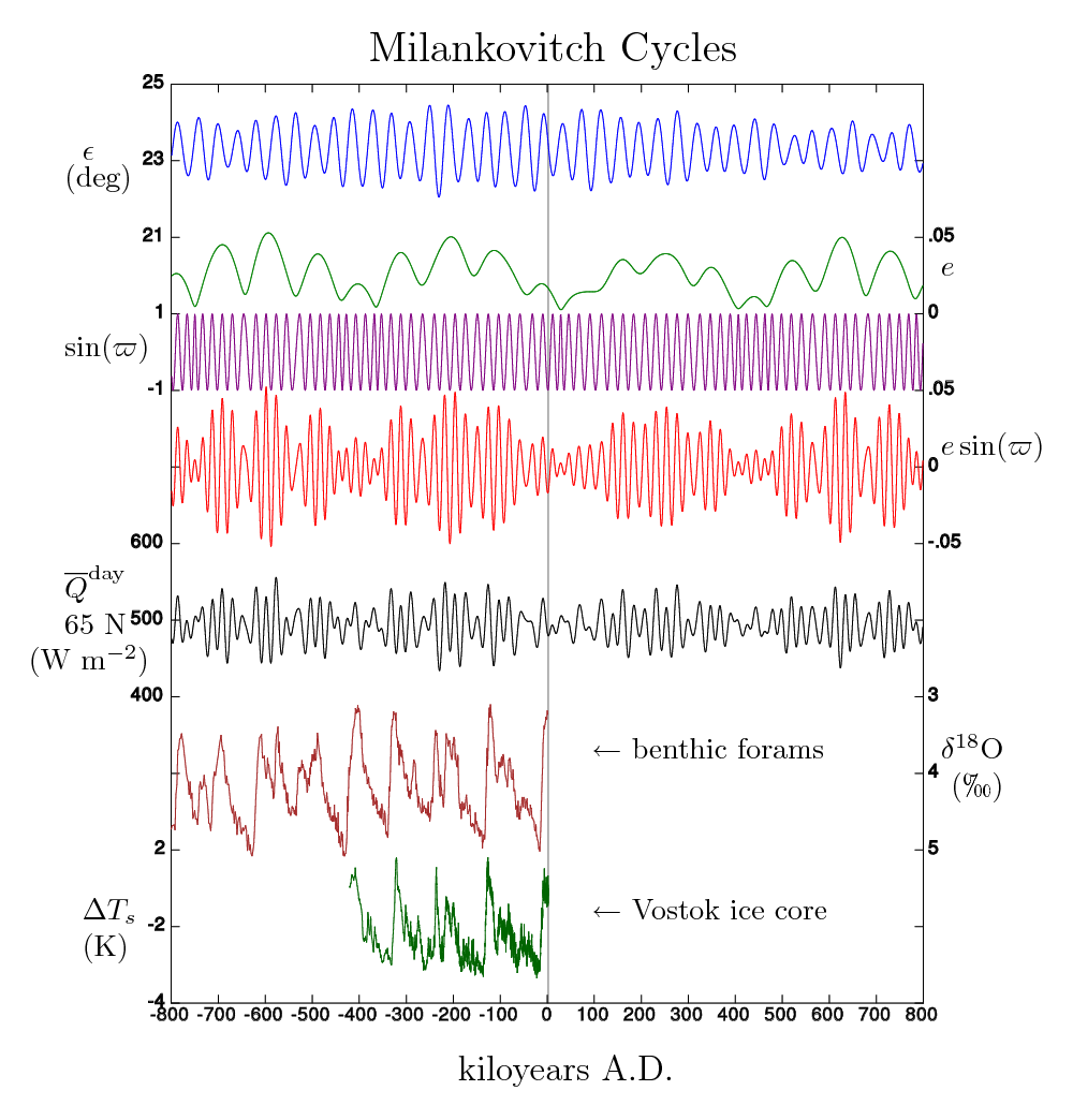
The first curve (blue) shows the changes in the Inclination of the Ecliptic, ε. The second curve (green) indicates the much slower changes in the Earth's eccentricity, e. And, the third curve (purple) gives the changes in the angle of perihelion.
Local heating depends on the angular distance of the Sun from the local zenith and so is a function of the Sun's apparent inclination and the number of hours of daylight. At any given time the Earth may not be exactly in equilibrium with the current heating conditions. Looking at the "number of days of heating" and the changes that are taking place might give a better picture of what is happening than one might get from the integrals in the Wikipedia article on insolation.
Supplemental (Aug 10): The calculation didn't take into consideration changes in the semi-major axis, a, which would affect the mean motion and the length of the year. In perturbation theory the semi-major axis is considered an adiabatic invariant. This would justify the first coefficient in the formula being a constant rather than a function of the eccentricity, e.

Note that the number of days between the equinoxes can vary by as much as 25 days. The image below is from the Wikipedia article on Milankovitch cycles.
The first curve (blue) shows the changes in the Inclination of the Ecliptic, ε. The second curve (green) indicates the much slower changes in the Earth's eccentricity, e. And, the third curve (purple) gives the changes in the angle of perihelion.
Local heating depends on the angular distance of the Sun from the local zenith and so is a function of the Sun's apparent inclination and the number of hours of daylight. At any given time the Earth may not be exactly in equilibrium with the current heating conditions. Looking at the "number of days of heating" and the changes that are taking place might give a better picture of what is happening than one might get from the integrals in the Wikipedia article on insolation.
Supplemental (Aug 10): The calculation didn't take into consideration changes in the semi-major axis, a, which would affect the mean motion and the length of the year. In perturbation theory the semi-major axis is considered an adiabatic invariant. This would justify the first coefficient in the formula being a constant rather than a function of the eccentricity, e.
Empirical Formula for #Days Between V. Equinox & A. Equinox
I used different values for the eccentricity of the Earth's orbit, e, to get a set of values for the coefficients of the formula found last time. A turned out to be a constant equal to half the number of days in the year and B was a simple function of e. θ is the angle of Earth's perihelion from the direction of the Winter Solstice in the Earth's orbital plane or 90° behind the Vernal Equinox.

I labeled the function for the number of days from the Vernal Equinox to the Autumnal Equinox VEq2AEq. The empirical error bound is a simple cubic function within the range of e for the formula, 0 < e < 0.07.
Supplemental (Aug 10): The polynomial fit for B(e) had some near zero values so I tried doing a least squares fit for just odd powers of e and got a better fit.
The rms error was 2·10-10. The function appears to be,
B(e) = 232.520·(e - e3/3! - 3e5/5! + ···).
First Order Approximation For #Days of Summer
To first order the number of days in Summer function for apsidal precession is a constant plus a cosine function. ΔΔt, the error for the approximation, has a magnitude less than 0.0003 days.

As before θ is the angle between the Earth's perihelion and the Winter Solstice. Apsidal precession has to be considered as a contribution to global warming. If there is net annual heating due to apsidal precession then this contribution needs to be deducted before the effect of greenhouse gases can be determined. Only the change in the angle of angle of perihelion was taken into consideration and the other orbital elements were assumed to remain constant.

As before θ is the angle between the Earth's perihelion and the Winter Solstice. Apsidal precession has to be considered as a contribution to global warming. If there is net annual heating due to apsidal precession then this contribution needs to be deducted before the effect of greenhouse gases can be determined. Only the change in the angle of angle of perihelion was taken into consideration and the other orbital elements were assumed to remain constant.
Monday, August 8, 2011
Conclusion: 30° Months Probably Not Practical
Defining a month as the time that it takes for the Earth to move 30° in its orbit is likely not practical since it would require frequent changes to keep the months accurate. The dates of apsides, equinoxes and solstices are something better to relocate to an almanac. The same for the number of days of net heating which I have referred to as "summer". It's probably best not to overcomplicate the calendar. One can just as easily draw attention to the perihelion by making it an "Earth day" holiday.
So, what to do about the months? The 7/12ths trick might be useful. Simplifying the day-of-year function would make it easier to compute the number of days between two dates such as the time between one equinox and the next.
When making changes that affect a lot of people it's probably best to adopt a minimalist approach.
The Equinoxes divide the year into two parts. When the Sun is above the Equator there is relatively more warming during this "half" of the year than when it is below it. There doesn't seem to be any collective terms for Spring/Summer and Fall/Winter. But the Earth's heat balance is positive for the former since the temperature rises and negative for the later since it decreases as a study of the Earth's insolation and climate models show. What is often overlooked or downplayed is that there are indeed long term changes over time.
Adjusting the Months to Fit the Earth's Orbidal Motion
If we wanted the Tropical Calendar to be a "Global Warming Calendar" we might adjust the number of days in each month to better fit the orbital motion of the Earth. We could make the length of each month correspond to a change of 30° relative to the Vernal Equinox. We would want the year to start in mid winter so the year would have to begin at the Winter Solstice or perhaps the next day.

Each of the months above fit this pattern with a Solstice or Equinox separating a block of three months. We could add the leap day at the end of the year where it was at one time or perhaps add it just before the Vernal Equinox to mark its significance as the date which we use to synchronize the calendar with the tropical year.
As the date of perihelion moves about in the year during the apsidal precession cycle periodic "calendar reforms" would be necessary to correct the lengths of the months to maintain the pattern of 30° monthly steps. It might be practical to do this every 1/12th of the 20,934 tropical year apsidal cycle which is about 1744 tropical years*. Leaving the calendar design somewhat open ended would allow changes to be made as our understanding of these changes increases and keep the calendar from becoming something rigidly preordained.
Supplemental: Basing the lengths of the months on the Earth's orbital motion was intended to focus attention of the Earth's heat balance and changes over time. There is a seasonal lag so temperatures do not exactly match the "seasons" but the highs and lows are delayed somewhat.
*Supplemental: Perihelion moves about 8.8° in 512 tropical years and 2.2° in 128 years. 512 years might be a little long to keep the system accurate and there is the problem of keeping people's interest in updating the calendar over that long a span of time. 128 years is more convenient because it could be done when the leap year is skipped but rearranging the calendar that often is a problem for historians.
Sunday, August 7, 2011
Apsical Precession & the Length of Summer
Apsidal precession causes small changes in the length of Summer as the images below show. The plot gives the number of days of from the Vernal Equinox to the Autumnal Equinox as a function of the angle of perhelion from the Winter Solstice. The result is a peak-to-peak variation of about 8 days.

This is only a 2% change but could have a greater affect at higher latitudes where thermal cycling is the greatest.

If the perihelion is at midsummer one might expect a slightly greater intensity of solar radiation since the Earth would be closer to the Sun at this time of year. Winters in the Northern Hemisphere may on average be slightly milder at this time than at other times in the 21,000 year apsidal precession cycle. The apsidal precession is barely noticeable since it is masked by the shifts caused by a leap day every four years. It takes on average about 57.5 years for the date of perihelion to move one day backwards in the year so it may be just noticeable within the span of a lifetime.
Saturday, August 6, 2011
The Earth's Apsides & Long Term Climate Change
The proposed calendar change would help fix the dates of the equinoxes and solstices better but the perihelion and aphelion of the Earth's orbit will still move about within the year. The process involved is known as apsidal precession. I've computed the rate of motion of the equinoxes within the Julian calendar and the rate of apsidal precession for the Julian, Gregorian and "Tropical" calendars. The "P"s are the periods or "days per year" and the "n"s are the rates of the mean motions.* One can use the relative difference in rates to find the period of the cycle since dividing by a rate is equivalent to multiplying by the length of its year.
 (click to enlarge)
This prcession will affect the motion of the Sun within the year and consequently the length of the seasons since the Earth moves faster in its orbit near perihelion and slower near aphelion. The lengths of summer and winter are an important factor in long term climate change.
*Edit: The subscript "a" refers to the anomalistic year which is the time between one perihelion and the next. It is slightly different than the time between successive Vernal Equinoxes.
Supplemental: With apsidal precession one could "fix" the date of the Vernal Equinox but the Autumnal Equinox and the solstices would vary slightly relative to it over time due to changes in the length of the seasons. All the dates would still vary over a four year period because of the leap day.
Historical Values for the Tropical Year Converted to Alternating Series
If one converts the historical values for the tropical year into alternating unit fractions in which the numbers are multiples of each other it appears that Tycho Brahe was the first to get 365 + 1/4 - 1/128 days.
 Click to enlarge
Brahe's value for the tropical year, 365 days, 5 hours, 48 minutes, 45 seconds, can be found in Astronomiae Instauratae Progymnasmatum, Pt I (1602).
 Click to enlarge
Brahe's value for the tropical year, 365 days, 5 hours, 48 minutes, 45 seconds, can be found in Astronomiae Instauratae Progymnasmatum, Pt I (1602).
Friday, August 5, 2011
A More Practical Decision Tree
Division of the year by 128 is more difficult than division by 100 or 400 but in practice one could keep track of the year that is the next multiple of 128. Initially the next multiple is 2176.

As time passes and the year reaches the multiple the leap year is skipped and a new next multiple is determined. This simplifies the decision process by avoiding division by 128.

As time passes and the year reaches the multiple the leap year is skipped and a new next multiple is determined. This simplifies the decision process by avoiding division by 128.
Thursday, August 4, 2011
Simplied Decision Tree For Switch Between 2048 and 2100
I waw looking for a way to simplify the flowchart for the Alternative Calendar and noticed that there was a window of opportunity to adopt a simple decision tree between 2048 and 2100 since 2048 is exactly divisible by 128. The decision tree for the Gregorian Calendar is,

The simplified decision tree for the Alternative Calendar is,

The 52 year window allows us to use the year instead of a difference in years in the decision tree. Both decision trees give the same results within this window.

The simplified decision tree for the Alternative Calendar is,

The 52 year window allows us to use the year instead of a difference in years in the decision tree. Both decision trees give the same results within this window.
Comparision of the Flowcharts for Determining Leap Years
I used MS Word 2003 to do create the flowcharts needed to determine when a year is a leap year for the Gregorian Calendar and the proposed Alternative Calendar. There is one step less for deciding in the Alternative Calendar which shows that this calendar is simpler. At the decision points in the flowcharts the "mod" used is the modulo operator.

The Gregorian Calendar was introduced in late 1582. It was noticed that the Vernal Equinox was shifting relative to the Julian Calendar so a new calendar was devised. This was just prior to the year 1600 which was the last year of the 399th quadrennium, the four year leap year cycle. It was a convenient time to initiate the centennial leap year cycle.

There were other factors that were taken into consideration is developing the Gregorian Calendar. For example the number of days in the 400 year cycle of the calendar is exactly divisible by 7 and the cycle of the weeks will then repeat itself. The Alternative Calendar ignores lunar cycles but it may be possible do something similar for the Lunar Calendar and develop a simple set of rules for it too.
Edit: Corrected the errors involving the year in the Gregorian Calendar Flowchart
Supplemental: The procedure for the Alternative Calendar can be simplified by working in the new system and noting that 2048 is exactly divided by 128. See next blog.
Wednesday, August 3, 2011
A Simple Set of Rules for Leap Years
The Wikipedia article on the tropical year gives a more accurate value for the mean number of days in a year than was previously used. It would also be more convenient to make the period of a correction a multiple of the previous period. This was a fluke for the alternating series composed of unit fractions.

As one can see this works quite well for the mean length of the year. A limit on the usefulness of any calendar and its set of rules results from the changing length of the day which decreases by about 1.5 msec per century. Using the first two fractions would probably be the best correction to make at this time. In making changes we also need to consider the convenience of decision points and the ease of transition from one set of rules to another. We have a window of opportunity to make such a change before the year 2100. The rules for the Gregorian calendar are good for approximately 3200 years and the change isn't actually necessary. It would just be a matter of convenience. Should we give the World an opportunity to decide or just let it ride?

As one can see this works quite well for the mean length of the year. A limit on the usefulness of any calendar and its set of rules results from the changing length of the day which decreases by about 1.5 msec per century. Using the first two fractions would probably be the best correction to make at this time. In making changes we also need to consider the convenience of decision points and the ease of transition from one set of rules to another. We have a window of opportunity to make such a change before the year 2100. The rules for the Gregorian calendar are good for approximately 3200 years and the change isn't actually necessary. It would just be a matter of convenience. Should we give the World an opportunity to decide or just let it ride?
Monday, August 1, 2011
Efficient Rules & A Proposed Calendar Reform
Too much dissent is likely to be harmful to a nation and can disrupt the government's need to make decisions. But we also need to consider the quality of the decisions made. Let's assume that a given rule has a given lifetime. Change within that lifetime is unnecessary and arbitrary change may be considered a nuisance. So we might approach the problem from the perspective of least action.
Let us look at calandar reform as an example. The Julian Calendar adopted 365 + 1/4 days for the year. It was found that this led to a deviation from the natural year or the mean time between equinoxes. The Gregorian Calendar corrected this and adopted a mean year of 365 + 1/4 - 1/100 + 1/400 days. But it turns out that this system does not result in the most efficient set of rules.
The value that The Explanatory Supplement to the Astronomical Almanac gives for the mean number of days per year is 365.2421897. There are a number of ways of representing a fraction one of which is continued fractions. The number of terms in the continued fraction can be terminated after a given number of terms and can be converted to a mixed fraction. This simplifies the design of gear trains which can reproduce a given ratio. A simplier system is that of a series of alternating unit fractions. Each unit fraction tells us how frequently we have to break the set of rules defined by the subset of unit fractions. The sequence of alternating unit fractions that corresponds to the number of days in a year is 365 + 1/4 - 1/128 + 1/454545...

Evaluating the expressions for the various number of days in a year shows that even two terms of the alternating unit fraction provides a better approximation for the actual number of days in a year than that does the Gregorian Calendar. So we may ask if all the hassle of Y2K was really necessary. One might conclude that the Catholic Church, the scientific community and government are all "fallible" to some extent.
It might be wise to consider alternatives to this set of rules but if the world wanted to this calendar reform could be adopted by the United Nations and approved by individual nations. A nominal starting year would be the year 2001* since the new proposal and the Gregorian Calendar agree on leap years until the year 2100.
*Edit: You would need to count the number of years from the year 2000 and base the decision for the leap day on whether the number of years is zero modulo 4, 128 (, etc.)
Wednesday, July 27, 2011
Some Readings on the Debt Crisis
2011 U.S. Debt ceiling crisis
Sovereign default
Government budget deficit
United States public debt
United States federal budget
Cost-benefit analysis
Multiplier (economics)
Fiscal multiplier
Inflation
Diminishing returns
Debt management plan
Financial crisis
Crisis management
Obstructionism
Brinkmanship
Leverage (negotiation)
Compromise
Manufactured crisis
Sunday, July 24, 2011
An Ancient Egyptian Leveling Tool
In Ancient Egypt an A-shaped wooden frame with a plumb bob was used as a leveling tool. It was known as a khekh. An example of this is the triangle level found in the tomb of Sennedjem from the 19th dynasty.
 Source: Budge, An Egyptian Hieroglyphic Dictionary
 Source: Budge, An Egyptian Hieroglyphic Dictionary
The Bouguer Anomaly
The Bouguer Anomaly is a contribution to the deviation from vertical caused by irregularities in the Earth's gravitional field due to variations in density. It is most noticable near mountainous regions where it can be on the order of one minute of arc. Changes in altitude also result in gravity anomalies since gravitation is a function the distance from the Earth's center. Gravity anomalies have been known for a long time.The Schiehhallion Experiment of 1774 which involved the gravitational deflection caused by a mountain in Scottland which was used in an attempt to measure the mean density of the Earth and hence the gravitational constant.
Monday, July 18, 2011
Galileo Satellite Navigation System
The European Galileo satellite navigation system is about to enter a new phase that of in-orbit validation (IOV). The first IOV satellites are due to be launched within the next year and will enable ESA to test the satellite and ground station systems before the entire constellation of satellites is placed in orbit. This is the topic of a recently released ESA video.
Monday, July 11, 2011
ERS-2 Images of the Kangerdlugssuaq Ice Stream
ESA has recently posted ERS-2 images of the Kangerdlugssuaq ice stream in Greenland which is advancing at 35 meters per day.
 Credits: ESA
There are claims that this is due to global warming but one should also note that Greenland has many hot springs and these may be a contributing factor. This part of Greenland faces Iceland which has experienced some recent volcanic eruptions. Global warming produces the greatest temperature increase in the Artic which can be seen by the decline of the northern ice pack. Climate changes slowly over time and a retreat of the glaciers has been taking place over the 10,000 years since the last glacial period when much of the northern hemisphere was covered by ice sheets.
Supplemental readings: Glacial meltwater, Subglacial lake, Jökulhlaup, Meltwater pulse 1A, Tunnel valley, fjord, glacial valley. (Is history repeating itself? One gets the impression that ice sheets and glaciers have rather complicated mechanisms associated with them.)
Credits: ESAThere are claims that this is due to global warming but one should also note that Greenland has many hot springs and these may be a contributing factor. This part of Greenland faces Iceland which has experienced some recent volcanic eruptions. Global warming produces the greatest temperature increase in the Artic which can be seen by the decline of the northern ice pack. Climate changes slowly over time and a retreat of the glaciers has been taking place over the 10,000 years since the last glacial period when much of the northern hemisphere was covered by ice sheets.
Supplemental readings: Glacial meltwater, Subglacial lake, Jökulhlaup, Meltwater pulse 1A, Tunnel valley, fjord, glacial valley. (Is history repeating itself? One gets the impression that ice sheets and glaciers have rather complicated mechanisms associated with them.)
Sunday, July 3, 2011
Earth at Aphelion on the 4th of July
MICA, the US Naval Observatory's Multiyear Interactive Computer Almanac, indicates that the Earth will be at aphelion, the furthest distance from the Sun, on 4 July 2011 at about 14:54 UT.

The terms perihelion and aphelion were first used in connection with the epicycle discription of the motion of the Sun, Moon and planets referring to points in their orbits so these concepts may be over 2000 years old. Ptolemy uses the terms "perigee" and "apogee" since his epicycle orbits were centered on the Earth. The composite motion of epicycle and deferent is somewhat elliptical and are a good approximation to the motion of the Sun and Moon so it is not surprising that there are near and far points in these "orbits." Ptolemy gives Gemini 5° 30' or 65° 30' for the position of the Sun's apogee.
Supplemental: When comparing Kepler's elliptical orbits with Ptolemy's epicycles it might be fairer to think in terms of the relative motion of the Sun and the Earth. According to Archimedes, Aristarchus postulated that the Earth circled the Sun circa 300 BC. Ptolemy may have been aware of this since he had access to Archimedes (see Almagest p. 44). It is probably best to separate observations from theory as much as possibly to avoid contaminating them with errors unnecessarily. Especially when the observations are solely Earth based.
Subscribe to:
Posts (Atom)